About
Randy Krum
President of InfoNewt.
Data Visualization and Infographic Design

Infographic Design

Infographics Design | Presentations
Consulting | Data Visualizations

DFW DataViz Meetup

Join the DFW Data Visualization and Infographics Meetup Group if you're in the Dallas/Fort Worth area!

Search the Cool Infographics site

Custom Search

Subscriptions:


Feedburner

The Cool Infographics® Gallery:

How to add the
Cool Infographics button to your:

Cool Infographics iOS icon

- iPhone
- iPad
- iPod Touch


Read on Flipboard for iPad and iPhone

Featured in the Tech & Science category

Flipboard icon

Twitter Feed
From the Bookstore

Caffeine Poster

The Caffeine Poster infographic

Entries in map (184)

Tuesday
Aug162016

Animated and Interactive Global Shipping Visualization

This is a fantastic detailed animated and interactive data visualization of the world's Global Shipping Traffic.

You can see movements of the global merchant fleet over the course of 2012, overlaid on a bathymetric map. You can also see a few statistics such as a counter for emitted CO2 (in thousand tonnes) and maximum freight carried by represented vessels (varying units).

The merchant fleet is divided into five categories, each of which has a filter and a CO2 and freight counter for the hour shown on the clock. The ship types and units are as follows:

  • Container (e.g. manufactured goods): number of container slots equivalent to 20 feet (i.e. a 40-foot container takes two slots)
  • Dry bulk (e.g. coal, aggregates): combined weight of cargo, fuel, water, provisions, passengers and crew a vessel can carry, measured in thousand tonnes
  • Tanker (e.g. oil, chemicals): same as dry bulk
  • Gas bulk (e.g. liquified natural gas): capacity for gases, measured in cubic metres
  • Vehicles (e.g. cars): same as dry bulk

The map was created by Kiln based on data from the UCL Energy Institute (UCL EI)

You can hide the route lines and just watch the ship dots move over time. It's mezmerizing!

Thanks to Jim Hopkinson and Bill Gates for sharing on Twitter!

You can see the interactive version embedded here, or click here to take you to the full-size original site:


Wednesday
Jul132016

Global Connectivity Ranking

Global Connectivity Ranking interactive infographic world London

The Global Connectivity Ranking from Rome2rio includes a beautiful interactive data visualization showing how connected we are on a global scale. Above you can see the direct flight connections from London, the most connected city on Earth.

Just how connected are our cities?  How do we measure such connections?  How do these connections change over time?

To answer these questions, my research team at KPMG collaborated with Rome2rio to produce the Global Connectivity Ranking. We ranked all 1,212 cities on the planet which operate international airports.

The Rome2rio Global Connectivity Ranking reflects the number of international cities that a city is connected to through direct flights. It measures connections from city to city - not airport to airport. For example, the connection count for London reflects how many cities outside the UK that can be reached from any of London's 6 international airports. Rankings were computed using Rome2rio's global transit data from April 2014 and January 2016.

Choose any city on the list to animate to direct flight connections. The size of the bubbles over each city also represent the total number of connections from that city.

The default is the world view, but can also choose to focus on a single continent. Here you can see the connection from Chicago when zoomed in to only North America.

Global Connectivity Ranking interactive infographic North America Chicago


Wednesday
Jun292016

The U.S. MiseryMap of Flight Delays

The U.S. MiseryMap of Flight Delays Map Infographic

Stuck in an airport? The MiseryMap from FlightAware shows a real-time view of flight delays and cancelations at the top 30 airports in the U.S.

Doughnut charts highlight the totals for each major city (combining airports if there are multiple) and hovering or clicking a specific city will show the flight routes (sankey diagram style) that are experiencing delays and cancelations. The full details are shown in the barr chart sidebar.

Pressing the play button will animate the map for the last 48 hours showing the changes to the weather map overlay, and delays in 4-hour increments. The overall size of each doughnut also seems to represent the total number of flights from that city in each 4-hour increment.

The U.S. MiseryMap of Flight Delays Map Infographic DFW

Thanks to Mary Kaye for sharing the link!

Friday
Jun242016

How Britain Voted in the E.U. Referendum

How Britain Voted in the E.U. Referendum map infographic

Britain voted on Thursday to part ways with the European Union. The vote was incredibly close, and this choropleth map visualization from the NY Times tells an intriguing story.

Britain has voted to leave the European Union, a historic decision sure to reshape the nation’s place in the world, rattle the Continent and rock political establishments throughout the West.

The margin of victory startled even proponents of a British exit. The “Leave” campaign won by 52 percent to 48 percent. More than 17.4 million people voted in the referendum on Thursday to sever ties with the European Union, and about 16.1 million to remain in the bloc.

Britons voted on Thursday to leave the European Union. The Leave side led with 17.4 million votes, or 52 percent, versus the Remain side’s 16.1 million, or 48 percent, with a turnout of around 72 percent.


Friday
Jun032016

The Global Air Transportation Network

The Transportation Clusters infographic is a force-directed map of the 3,275 global airports and all of the connecting flight routes. Designed by Martin Grandjean, each bubble represents an individual airport and the bubble sizes represents the number of flight routes (37,153 routes in total) based on OpenFlights.org data.

People travel not just more frequently, but increasingly far and quickly. Mapping the connections between all the airports worldwide is a fascinating network visualization exercise.

This post (which may be followed by further experimentations in this area) is an attempt to make explicit the network behind air transport. The structure of the relationships has an impact on the spatial distribution of nodes in a graph. Let’s see how this landscape is reorganized without geographical constraints.

This “map” is the result of the application of a force-directed layout algorithm on a graph of 3.275 airports (37.153 single routes – the weighted total is higher because many airlines take the same route), based on OpenFlights.org data. Naturally, network geography is not completely disrupted: the continents are mostly visible and regions are generally in their original position (with the exception of the Pacific islands that connect Asia and America – imagine this graph in three dimensions, with the Pacific Ocean behind). Major observations: India is more connected to the Middle East than to South and East Asia. The Russian cluster is very visible, connecting airports in Russia but also in many former Soviet republics. Latin america is clearly divided between a South cluster and a Central American cluster very connected with the U.S.

The force-directed layout spaces the bubbles apart so there are no overlapping bubbles. The color coding is a color spectrum based on longitude, and generally groups airports from the same continent together. The total number of flights is much higher than the number of routes because many airlines share the same routes. I would like to see a version that weights the connecting lines with the number of flights that share that same route.

Here you can see the original map with the bubbles accurately located geographically, but a lot of overlap based on close proximity of the airports:

Martin also published a cool animated GIF and YouTube video of the change from geographical to force-directed layout.


Found on FlowingData

Friday
May132016

American Slavery Maps

American Slavery Maps Infographic

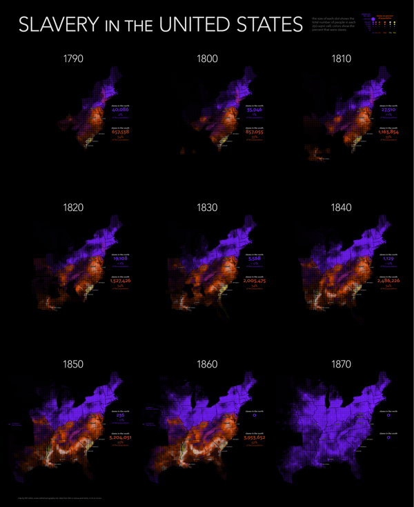
Bill Rankin at Radical Cartography has created nine uniform grid maps of American Slavery covering each decade from 1790 to 1870. I've combined them into the animated GIF you see above. Bill took a new approach in analyzing the historical data by 250 square mile units instead of the traditional data by county.

The gradual decline of slavery in the north was matched by its explosive expansion in the south, especially with the transition from the longstanding slave areas along the Atlantic coast to the new cotton plantations of the Lower South. And although the Civil War by no means ended the struggle for racial equality, it marked a dramatic turning point; antebellum slavery was a robust institution that showed no signs of decline.

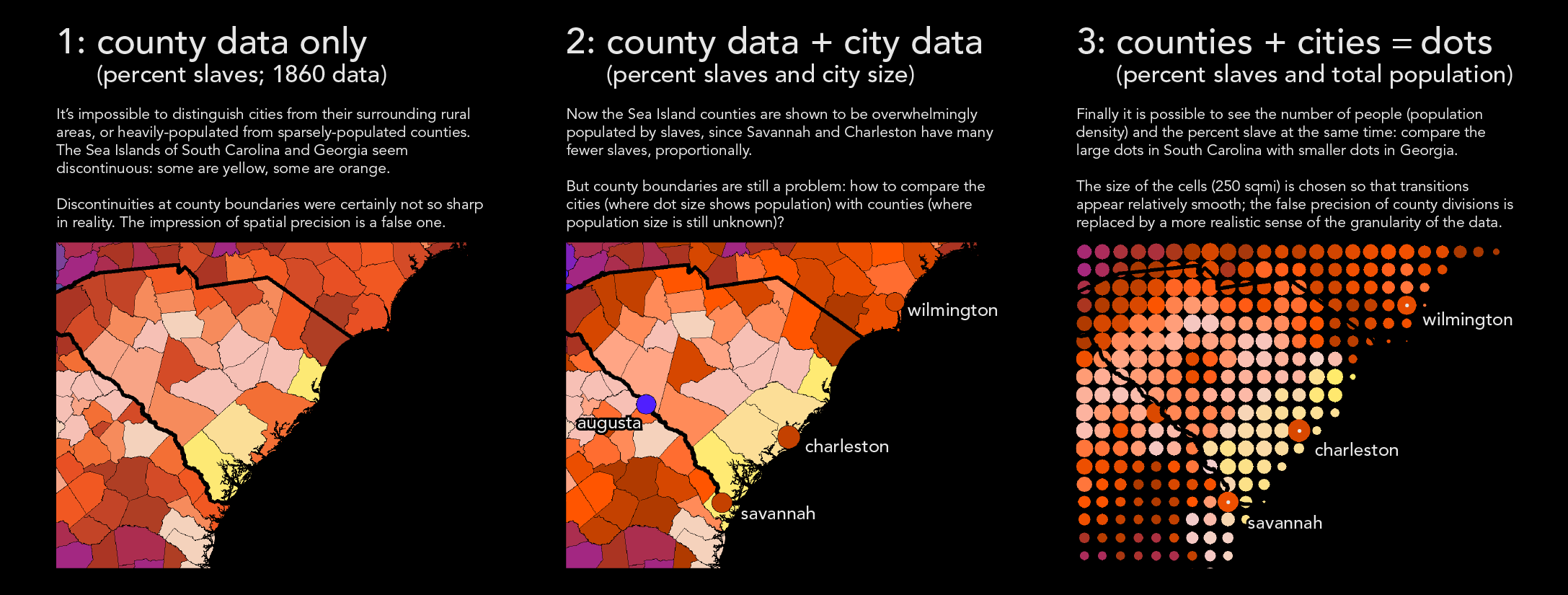
Mapping slavery presents a number of difficult problems. The vast majority of maps — both old and new — use the county as the unit of analysis. But visually, it is tough to compare small and large counties; the constant reorganization of boundaries in the west means that comparisons across decades are tricky, too. And like all maps that shade large areas using a single color, typical maps of slavery make it impossible to see population density and demographic breakdown at the same time. (Should a county with 10,000 people and 1,000 slaves appear the same as one that has 100 people and 10 slaves?)

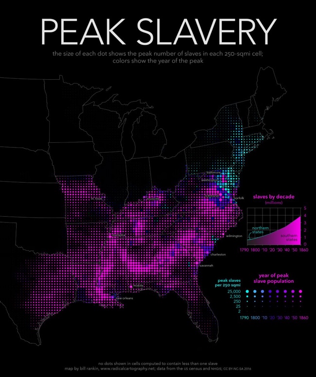
My maps confront these problems in two ways. First, I smash the visual tyranny of county boundaries by using a uniform grid of dots. The size of each dot shows the total population in each 250-sqmi cell, and the color shows the percent that were slaves. But just as important, I've also combined the usual county data with historical data for more than 150 cities and towns. Cities usually had fewer slaves, proportionally, than their surrounding counties, but this is invisible on standard maps. Adding this data shows the overwhelming predominance of slaves along the South Carolina coast, in contrast to Charleston; it also shows how distinctive New Orleans was from other southern cities. These techniques don't solve all problems (especially in sparsely populated areas), but they substantially refocus the visual argument of the maps — away from arbitrary jurisdictions and toward human beings.

For a graphic explanation of this technique, see here.

I appreciate him explaining his map technique! Each decade is a separate high-resolution map image, but Bill also created a fantastic combined map showing the highest Peak Slavery levels of slavery throughout the entire time period.

The bottom map shows the peak number of slaves in each area, along with the year when slavery peaked. Except in Delaware, Maryland, and eastern Virginia, slavery in the south was only headed in one direction: up. Cartographically, this map offers a temporal analysis without relying on a series of snapshots (either a slideshow or an animation), and it makes it clear that a static map is perfectly capable of representing a dynamic historical process.

American Slavery Peak Map


Additionally, you can download a high-resolution poster version showing all nine decades:

American Slavery Maps Poster


 Found on FlowingData and CityLab

Tuesday
Dec292015

Where The USA Gets Its Oil

Where The USA Gets Its Oil infographic

Two data visualization maps from Aschere Energy Education that show Where The USA Gets Its Oil.

The area cartogram created with a Gastner-Newman diffusion based algorithm is used to resize the countries above. It's a fun and unusual visualization method that stands out and gets attention because it breaks our usual understanding of the world map.

The second map uses the 3D heights of the countries and color-coding to represent the oil & petroleum exports to the U.S.

Thanks to Joe for sending in the link!

Monday
Jul202015

Beautiful Map Posters of Anywhere

Mapiful custom map posters

Mapiful is a great site that lets us choose the location and customize a beautiful black & white poster of any location in the world based on OpenStreetMap data. You can change the location, the zoom level, the label text, the orientation, and choose from a handful of clean layout styles.

The printed posters are a flat cost of $60 with free shipping worldwide.

Regardless of where you live and what city, country or spot you wish to eternalize - Mapiful takes you there. We bring people's favorite places to their homes. The city you were born, where you fell in love or just a place that makes your heart skip a beat. Search, zoom and tweak. Within days your unique Mapiful print will arrive in the mail.

Found on FlowingData and Visual News

Wednesday
May062015

Gardening Hardiness Zones

Gardening Hardiness Zones infographic

When planting a garden, it is best to understand which crops will preform best in different climate zones. Avant Gardening has developed the Gardening Hardiness Zones infographic for the gardener in any part of the United States.

We love the changing seasons, but we definitely miss spending time in our gardens. Every winter, we are starting to wonder when we can begin planting again. 

So, when can we get back out there? The best time for starting your garden depends on where you live. That’s why every gardener knows their USDA Plant Hardiness zone.

A hardiness zone, as defined by Wikipedia, is a “geographically defined area in which a specific category of plant life is capable of growing, as defined by climatic conditions, including its ability to withstand the minimum temperatures of the zone.” 

The USDA sets the zones based on the average annual extreme minimum temperature during a 30-year period in the past. The zones are not determined by the lowest temperature that has ever occurred or what is predicted to occur.

Know Your Hardiness Zone

So, how do you know which zone you’re in? The USDA has created a very detailed map outlining the US and how the zones are broken down. This resource is second-to-none when it comes to hardiness zones.

Once you determine in which hardiness zone you reside – and it is as simple as visiting the USDA map and clicking the mouse on your location - you can use this information to better plan your garden. 

Thanks to Deirdre for sending in the link!

Friday
Jan232015

Equal Population Mapper

Equal Population Mapper Interactive Infographic

Ben Blatt has created the Equal Population Mapper infographic. The interactive version at Slate.com allows you to choose New York City, Los Angeles County, Wyoming, New Jersey, Texas, or the Coastal regions as the target population. Then you select anywhere else on the map and a red circle will appear to show how big of an area you would have to select to have an equal population to your selection.

If you throw in New York City’s other four boroughs, the Big Apple’s total population is just greater than 8 million. That’s about the same number of people who live in Idaho, Montana, Wyoming, North Dakota, South Dakota, Nebraska, and the western half of Minnesota combined.

But don’t let my New York City–centric comparisons hinder your imagination. The interactive at Slate.com lets you visualize how different parts of the country compare in population density.

Click the button at the bottom of the interactive to select Los Angeles County, for instance, and then click anywhere on the map to generate a (roughly) circular region of (roughly) equal population. The population data come from the 2010 census, and the square mileage was calculated by summing each highlighted county’s total area. You can also use New Jersey (the most densely populated state), Wyoming (the least densely populated state outside of Alaska), Texas, the coasts (the group of all counties that come within 35 miles of either the Atlantic or Pacific oceans), and, yes, New York City as the baseline for your population comparison.

Cool interactive map!

Found on Flowingdata!